1. The Thurstone Model

The Thurstone Model

声明：本文为本人毕业研究报告《The Exploration of Pairwise Comparison in Football Application》中的部分内容摘录与整理，仅用于学习与交流。

Introduction

The method of paired comparisons, originally proposed by Thurstone [1], is a cornerstone of psychometrics and preference modeling. It provides a statistical framework for inferring psychological scales from pairwise choices or judgments.

Thurstone’s model is a method for sensory difference testing that ranks various stimuli on a perceptual scale for comparative analysis. In this model, a set of stimuli denoted as $O_1,O_2,\dots ,O_n$ are quantitatively compared based on the sensations $X_i$ they evoke in individuals. These sensations are assumed to be normally distributed across a population, with each $X_i$ lying on a sensation continuum $S$.

The sensation continuum $S$ serves as the quantitative scale on which these sensations are placed, with each sensation $X_i$ having an associated mean value $S_i$. This mean $S_i$ represents the average perceived intensity or preference of stimulus $O_i$ across the population, situating each stimulus on the continuum based on its evoked sensation’s mean.

The following model formulation encapsulates a concise mathematical summary of Frederick Mosteller’s [2] idea, transforming his conceptual research into a structured mathematical model.

Model Foundation

Given $X_i$ and $X_j$ as sensations evoked by the $i$th and $j$th stimuli, respectively, in an individual $I$, for a population of individuals, assume:

1. $X_i$ and $X_j$ are jointly normally distributed with parameters:
   • Mean of $X_i$ is $\mu (X_i)=S_i$ for $i=1,2,\dots ,n$.
   • Variance of $X_i$ is $Var(X_i)={\sigma }^2(X_i)={\sigma }_{X_i}^2$ for all $i=1,2,\dots ,n$.
2. The correlation between $X_i$ and $X_j$ is denoted by $\rho (X_i,X_j)={\rho }_{ij}=\rho$ and assumed to be the same for all pairs $(i,j)$ where $i,j=1,2,\dots ,n$ and $i\ne j$.

For each $i,j=1,2,\dots ,n$, $i\ne j$, a multivariate normal (or Gaussian) distribution for a 2-dimensional random vector $(X_i,X_j)$ can be defined as follows,

$$(X_i,X_j)\sim \mathcal{N}(\mathit{\mu },\mathbf{\Sigma })$$

where the joint mean $\mathit{\mu }$ is

$$\mathit{\mu }=\left[\begin{array}{c}{S}_i\\ S_j\end{array}\right]$$

and the joint covariance matrix $\mathbf{\Sigma }$ is

$$\mathbf{\Sigma }=\left[\begin{array}{cc}{\sigma }^2& \rho {\sigma }^2\\ \rho {\sigma }^2& {\sigma }^2\end{array}\right]$$

with ${\sigma }^2$ representing the common variance for all sensations and $\rho {\sigma }^2$ indicating the covariance between any two sensations $X_i$ and $X_j$, underpinned by the correlation coefficient $\rho$.

Remark:
Thurstone’s original Case V assumed zero correlation ($\rho =0$) among stimuli, but Mosteller [2] demonstrated that Case V also holds if all pairwise correlations are merely equal, i.e., ${\rho }_{ij}=\rho$ for all $i\ne j$. This relaxed condition is more reasonable in practical data analysis.

---

For further explanation of Model Foundation. The covariance of two random variables $X_i$ and $X_j$ is defined as:

$$Cov[X_i,X_j]=\mathbb{E}[(X_i-{\mu }_i)(X_j-{\mu }_j)]$$

where ${\mu }_i=\mathbb{E}[X_i]$ and ${\mu }_j=\mathbb{E}[X_j]$.

The correlation coefficient between $X_i$ and $X_j$ is defined as:

$${\rho }_{ij}=\frac{Cov[X_i,X_j]}{\sqrt{Var[X_i]\cdot Var[X_j]}}$$

where $Var[X_i]={\sigma }_{X_i}^2$ and $Var[X_j]={\sigma }_{X_j}^2$.

Since $Var[X_i]=Var[X_j]$, the denominator becomes

$$\sqrt{Var[X_i]\cdot Var[X_j]}=\sqrt{{\sigma }_{X_i}^2{\sigma }_{X_j}^2}={\sigma }^2$$

Thus,

$${\rho }_{ij}=\frac{Cov[X_i,X_j]}{{\sigma }^2}$$

where $Cov[X_i,X_j]=\rho {\sigma }^2$.

The joint covariance matrix is defined as:

$$\mathbf{\Sigma }=\left[\begin{array}{cc}{\sigma }_{X_i}^2& Cov[X_i,X_j]\\ Cov[X_j,X_i]& {\sigma }_{X_j}^2\end{array}\right]$$

Note that $Cov[X_i,X_j]=Cov[X_j,X_i]$, therefore, this simplifies to the previous form.

---

Now, we know the foundation of the model. However, there is an issue that has to be solved while building the model. Let’s look at Figure 1: there is $X_2<X_1$ when $S_1<S_2$, this variability is due to individual differences in perception and is captured by the standard deviation ($\sigma$) of the sensations.

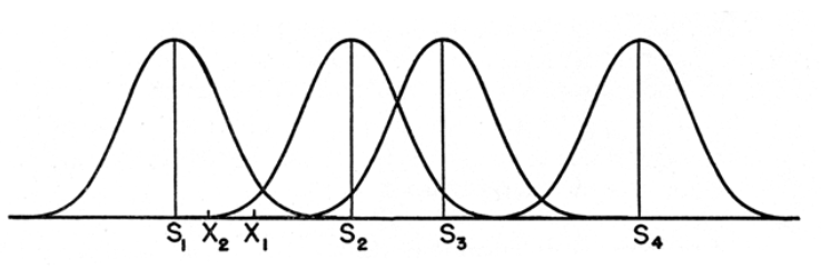
Therefore, when comparing two stimuli, individuals are required to make a definitive choice between them, so there is no tie in comparison. This binary (yes/no) outcome is crucial for determining the probability ($p_{ij}$) that one stimulus is perceived as stronger than the other.

The assumption is that in an idealized scenario, researchers know the exact proportion of times one stimulus is perceived as stronger than another. This knowledge allows them to precisely calculate the spacing of stimuli on the sensation continuum, reflecting not just the order in which stimuli are ranked but also the magnitude of differences between them.

Objective

Our aim is to determine the relative spacings of a set of stimuli, denoted by $S_1,S_2,\dots ,S_n$, on a sensation scale. These spacings are derived from probabilities $p_{ij}$, which represent the frequency at which a sensation evoked by stimulus i is preferred over that by stimulus j.

Note:
The scale values $S_i$ are only determined up to a linear transformation (i.e., they are relative positions), reflecting the inherent arbitrariness of the zero point and scale in psychological measurement.

Model Formulation 1

Let $X_i$ and $X_j$ denote the sensations evoked by the $i$th and $j$th stimuli, respectively, in an individual. These sensations are assumed to be jointly normally distributed across a population, with means $S_i$ and $S_j$, and a shared variance ${\sigma }^2$. The correlation between any two sensations $X_i$ and $X_j$ is denoted by $\rho$, assumed to be equal across all pairs of stimuli.

The probability of preference $p_{ij}$, i.e., the likelihood that sensation $X_i$ is greater than $X_j$, is calculated as:

$$p_{ij}=P(X_i>X_j)=\frac{1}{\sqrt{2\pi }\sigma (d_{ij})}{\int }_0^{\mathrm{\infty }}\exp \{-\frac{[d_{ij}-(S_i-S_j){]}^2}{2{\sigma }^2(d_{ij})}\}d{d}_{ij}$$

where

• $d_{ij}=X_i-X_j$ is the difference in sensations between stimuli $i$ and $j$.
• ${\sigma }^2(d_{ij})=2{\sigma }^2(1-\rho )$ defines the variance of the difference in sensations.

The integral calculates the area under the curve of the PDF for $d_{ij}$, adjusted for the mean difference in sensations $S_i-S_j$ and normalized by the variance of $d_{ij}$. The variance is normalized by setting $2{\sigma }^2(1-\rho )=1$.

To simplify for $p_{ij}$ with the normalized variance:

$$p_{ij}=\frac{1}{\sqrt{2\pi }}{\int }_{-(S_i-S_j)}^{\mathrm{\infty }}{e}^{-\frac{1}{2}{y}^2}dy$$

Given $p_{ij}$, $-(S_i-S_j)$ can be solved for using the standard normal distribution table. By setting $S_1=0$ as a reference point (a baseline), the relative mean sensations $S_i$ for all stimuli can be calculated.

Example 1

Consider a football scenario where we want to assess which of two players, Player A and Player B, might perform better in terms of goal scoring in a specific match based on their past performance. Assume their goal-scoring abilities are normally distributed sensations $X_A$ and $X_B$. $S_A$ and $S_B$ represent the average number of goals scored per match by Player A and Player B, respectively. Both have the same variability in their performance (${\sigma }^2$), and $\rho =0.5$ due to similar conditions.

Let:

• $S_A=0.8$
• $S_B=0.5$
• ${\sigma }^2=0.2$
• $\rho =0.5$

So, ${\sigma }^2(d_{ij})=2\times 0.2\times (1-0.5)=0.2$.

To find $p_{ij}=P(X_A>X_B)$:

$$S_A-S_B=0.3$$$$p_{ij}=\frac{1}{\sqrt{2\pi }}{\int }_{-(S_A-S_B)}^{\mathrm{\infty }}{e}^{-\frac{1}{2}{y}^2}dy$$

Using a standard normal distribution table, $p_{ij}\approx 1-\mathrm{\Phi }(-0.3)\approx 1-0.3821=0.6179$.
So, Player A has a 61.79% chance to score more than Player B.

Application:
The Thurstone model is widely used in product taste testing, consumer preference studies, psychological ranking tasks, and any context requiring conversion of paired choice data into a latent scale.

Model Derivation 1

Assume two normally distributed random variables $X_i$ and $X_j$ with means $S_i$ and $S_j$, and a common variance ${\sigma }^2$. The correlation between $X_i$ and $X_j$ is $\rho$. Define $d_{ij}=X_i-X_j$.

• Mean of $d_{ij}$:

$${\mu }_{d_{ij}}=\mathbb{E}[X_i-X_j]=S_i-S_j$$

• Variance of $d_{ij}$:

$${\sigma }^2(d_{ij})=Var[X_i-X_j]={\sigma }^2+{\sigma }^2-2\rho {\sigma }^2=2{\sigma }^2(1-\rho )$$

A random variable $Z\sim N(\mu ,{\sigma }^2)$ has PDF:

$$f(z)=\frac{1}{\sqrt{2\pi {\sigma }^2}}\exp \{-\frac{(z-\mu {)}^2}{2{\sigma }^2}\}$$

Apply to $d_{ij}$:

$$f(d_{ij})=\frac{1}{\sqrt{2\pi {\sigma }^2(d_{ij})}}\exp \{-\frac{[d_{ij}-{\mu }_{d_{ij}}{]}^2}{2{\sigma }^2(d_{ij})}\}$$

Compute the probability $p_{ij}=P(d_{ij}>0)$:

$$p_{ij}={\int }_0^{\mathrm{\infty }}f(d_{ij})d(d_{ij})=\frac{1}{\sqrt{2\pi }\sigma (d_{ij})}{\int }_0^{\mathrm{\infty }}\exp \{-\frac{[d_{ij}-(S_i-S_j){]}^2}{2{\sigma }^2(d_{ij})}\}d(d_{ij})$$

Now, to normalize variance, set:

$${\sigma }^2(d_{ij})=2{\sigma }^2(1-\rho )=1$$

This aligns the distribution with the standard normal $\mathcal{N}(0,1)$:

$$y=\frac{d_{ij}-(S_i-S_j)}{\sigma (d_{ij})}=d_{ij}-(S_i-S_j)$$

So, change of variable for the integration:

$$p_{ij}=\frac{1}{\sqrt{2\pi }}{\int }_{-(S_i-S_j)}^{\mathrm{\infty }}\exp \{-\frac{y^2}{2}\}dy$$

Conclusion

To sum up, the Thurstone model [2] is based on the idea of a continuum where each item (or stimulus) has a location that represents its "strength" or preference level. The probability of preferring stimulus $i$ over $j$ ($p_{ij}$) is modeled as the area under the normal distribution curve to the right of the difference in perceived strengths ($S_i-S_j$). This model inherently assumes that the differences in perceptions are normally distributed.

However, the Thurstone framework actually includes several "cases":

• Case V: Assumes equal variances and equal (often zero) correlations (as discussed here).
• Cases III and IV: Allow for unequal variances and/or unequal correlations; they are mathematically more general but computationally more complex [1,2].

However, the Thurstone model, while complex in its probabilistic approach to preference analysis, is limited by its dependence on a normal distribution and a constant correlation between stimuli. These assumptions may not hold in real-world scenarios, making the model computationally intensive and less suitable for large datasets or environments requiring quick decisions.

The simplified equation represents the prototype of the Bradley-Terry model [3], which resolves these issues by simplifying the distribution assumptions into a simple ratio-based model, enhancing both computational efficiency and applicability.

References

• [1] L.L. Thurstone. Psychophysical analysis. American Journal of Psychology, 38:368–389, 1927.
• [2] Frederick Mosteller. Remarks on the method of paired comparisons: I. The least squares solution assuming equal standard deviations and equal correlations. Psychometrika, 16(1):3–9, 1951.
• [3] Ralph Allan Bradley. Some statistical methods in taste testing and quality evaluation. Biometrics, 9(1):22–38, 1953.
• [4] J. P. Guilford. Psychometric Methods. McGraw-Hill Book Co., 1936.